Arcadia Collateral Risk Simulation: Progress Report 4
Arcadia Collateral Risk Simulation: Progress Report 4
Previous Reports
Report 1 - February 9
Report 2 - February 14
Report 3 - Feburary 21
In our previous progress report, we reviewed the simulation and validation processes to showcase how we ensure the simulation functions as intended. This week's report will dive deeper into the empirical borrower model and what the implications are on realism for the model.
This progress report is structured into four parts:
Empirical Borrower Model: A preview of the forthcoming update, focusing on a detailed exploration of the borrower data model and its implications for our simulation's realism and reliability.
Progress: A concise overview of the milestones reached and the enhancements made to the simulation during the current week.
Next Week's Goals: A forward-looking snapshot of our objectives to further refine the simulation's accuracy and scope.
Next Week’s Post: A preview of the forthcoming update, focusing on a simulation run on empirical data.
Empirical Borrower Distribution
The empirical borrower distribution provides an idea of borrower behavior in digital asset lending markets. This analysis shapes our simulation models by informing key assumptions and parameters when initializing the borrower model and creating a more realistic simulation. Through this, we gain essential insights into how a potential borrower can look in Arcadia.
Method 1: Total borrow vs Collateralization Ratio (CR) based on collateral vs numeraire token pairs.
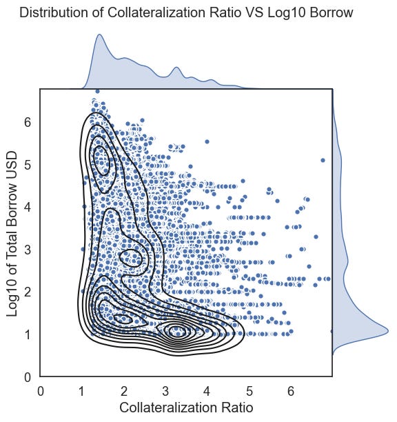
Method 1 entails a comparative analysis of total borrow amounts versus collateralization ratios (CR) for assets akin to collateral and numeraire token pairs at launch. It quantifies borrowing patterns by plotting loan amounts against CRs. It offers insight into lending behaviors of the reference protocol and acts as a proxy for Arcadia's future user base.
The chart above quantitatively analyzes the relationship between collateralization ratios and the log-transformed borrowing amounts in USD. The x-axis represents the Collateralization Ratio, a measure of the value of collateral provided for loans. The y-axis shows the borrowing amount on a logarithmic scale, enabling an adequate representation of a wide range of values.
Data points are dispersed across the chart, with contour lines indicating the density of these points. The concentration of data points within certain regions suggests common borrower behaviors and collateralization practices.
Marginal distributions on the top and right axes show the Kernel Density Chart of the Collateralization Ratios and borrowing amounts, respectively, offering a clearer view of their distributions.
Method 2: Empirical Distributions of Collateral for a given Borrow Position
For the second method, we apply a filter to identify borrow positions that involve a specific numeraire collateral asset pair, anticipated with the launch of Arcadia. Considering our reference protocol is a lending platform, borrowers may have several borrow positions against various types of collateral. This contrasts with an Arcadia Margin account, which permits borrowing of only one asset against a collateral set for any given Margin Account. To reconcile these differences, we adjust the size of each borrowed asset relative to the total borrowing and proportionately modify the collateral distribution to reflect this specific asset.
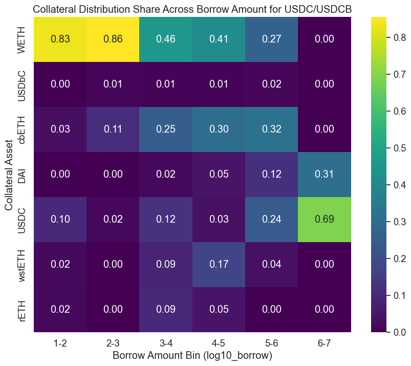
The chart above shows a heatmap visualizing the distribution of collateral types across different bins of borrow amounts (for a reference lending protocol) for USDC/USDCB. The x-axis represents the bins of borrow amounts, categorized by their log10 values ranging from 1 to 7. The y-axis lists various collateral assets. Each cell within the heatmap provides a proportional value, represented by both color intensity and a numeric label, indicating the share of a particular collateral type used for the corresponding borrow amount bin.
Key observations include:
WETH is prominently used as collateral, especially in lower borrow bins (1-2 and 2-3).
As the borrow amount increases, the use of cbETH as collateral grows, peaking in the 4-5 bin.
DAI and USDC see more usage as collateral in the higher borrow bins (5-6 for DAI and 6-7 for USDC).
This heatmap examines the patterns and preferences related to collateral among borrowers across various borrowing tiers within the lending platform. It provides insights into the potential distribution of borrowings for specific types of collateral. To initialize the borrower model, we have two approaches: we can predict the likely collateral distribution based on the size of the collateral sample, or we can directly draw samples from empirically observed borrower positions. Incorporating this element adds a layer of realistic borrower behavior to our simulation, thereby increasing its authenticity.
Goals for Week 8
For Week 8, the team is focused on the following objectives to develop further and refine our simulation model:
Completion of Week 7 Tasks: Finalize all remaining tasks from Week 7, ensuring that simulations cover all intended assets and LP tokens and that log visualization tools are fully operational.
Refinement and Optimization: Address the points for refinement and optimization identified during the previous week's work. This includes perfecting the simulation's parameters and enhancing the model's efficiency.
Improved Statistical Modeling: Begin coding the market impact simulations and develop statistical models to predict the asset holdings of generic accounts and to determine market scenarios for simulation. This phase is less about new code development and more about simulations, modeling, and analysis.
Initial Simulation Outputs: Generate the first set of outputs from the simulations, providing preliminary insights and data for review.
Progress Report:
As we conclude Week 7, our team has made substantial progress in advancing the simulation model, with a few objectives still being fully realized. Here is an overview of our achievements and ongoing efforts:
Comprehensive Simulation Coverage: We have partially expanded our simulations to include a broader array of single assets and LP tokens, integrating further time granularity. While we have yet to achieve all the changes we aimed for, significant strides have been made, and unforeseen fixes have been implemented on the fly.
Enhanced Log Visualization: Implementing advanced log visualization tools has seen partial completion. The tools currently in place have begun facilitating better data interpretation and are instrumental in tracking performance metrics. Further refinement is underway to realize the potential of these visualization capabilities fully.
Refined Borrower Models: We have successfully developed detailed borrower models based on the retrieved borrowing data. These models now accurately simulate a variety of risk profiles, offering a more nuanced understanding of borrower behaviors.
Expanded Testing: Our validation and verification testing has been partially carried out, focusing on aligning the model more closely with real-world scenarios. We continue to test and calibrate the model to ensure its accuracy and reliability.
Targeted Improvements: We have completed the targeted improvements set out for this week, enhancing the model's performance and resolving previously identified issues.
Next Week’s Post:
The upcoming post will present the first results of our simulation conducted on empirical borrower data. We will provide an analysis of the simulation's output. Stay tuned for a comprehensive overview of these insights.
Disclaimer: Any Materials presented here might change with the uncovering of new insights during simulation validation and verification.


